[Paper Review] NeurIPS 2017, Attention Is All You Need 논문리뷰

Attention Is All You Need

NeurIPS 2017

• 논문 링크: https://arxiv.org/abs/1706.03762
• github 링크: https://github.com/tensorflow/tensor2tensor

1. Introduction

Recurrent neural networks, long short-term memory and gated recurrent neural networks in particular, have been firmly established as state of the art approaches in sequence modeling and transduction problems such as language modeling and machine translation. → 문장처럼 순서가 중요한 데이터를 다루는 task에서는 RNN, LSTM, GRU가 가장 좋은 모델이었음.

 

Recurrent 모델은 input과 output의 순서를 봄. 그리고 t 시점에서의 hidden state h_t를 만들기 위해서는 previous hidden state h_t-1과 t시점의 input x_t가 필요함. → This inherently sequential nature precludes parallelization within training examples, which becomes critical at longer sequence lengths, as memory constraints limit batching across examples. → hidden state를 만드는 과정이 제한적이기 때문에 당연히 병렬 처리도 불가능하고, 정리하면 t=10 계산하려면 t=9가 필요하고, t=9 계산하려면 t=8이 필요함. → 동시에 못 돌림. → factorization tricks, conditional computation과 같은 방법으로 극복하려고 하기는 했지만, 여전히 sequential computation의 한계는 여전히 존재함.

 

Attention mechanisms have become an integral part of compelling sequence modeling and transduction models in various tasks, allowing modeling of dependencies without regard to their distance in the input or output sequences. → 그 이후 등장한 attention mechanism은 sequence나 transduction(변환) model에서 input과 output의 거리에 관계없이 쓰일 수 있음(Recurrent의 한계를 극복했다고 봐도 무방함.). 하지만, 여전히 Attention과 Recurrent 모델이 같이 쓰임(Attention + Recurrent).

 

In this work we propose the Transformer, a model architecture eschewing recurrence and instead relying entirely on an attention mechanism to draw global dependencies between input and output. → 순환 구조를 아예 쓰지 않음. → input, output 전체 범위의 의존성을 한 번에 모델링한다고 할 수 있음. → Recurrent과는 다르게 더 많은 병렬 처리가 가능함.

 

2. Background

The goal of reducing sequential computation also forms the foundation of the Extended Neural GPU, ByteNet and ConvS2S, all of which use convolutional neural networks as basic building block, computing hidden representations in parallel for all input and output positions. → 모든 위치의 token을 병렬로 처리할 수 있다는 장점이 있음. → 다만, 두 토큰이 멀리 떨어질수록 그 관계를 연결하려면 더 많은 연산 단계가 필요함(ConvS2S는 거리 늘수록 선형적으로 연산 증가, ByteNet는 거리 늘수록 로그 형태로 증가.) → 그래서 결과적으로는, 멀리 떨어진 단어 간의 관계를 배우기 어려움.

 

In the Transformer this is reduced to a constant number of operations, albeit at the cost of reduced effective resolution due to averaging attention-weighted positions, an effect we counteract with Multi-Head Attention as described in section 3.2. → 두 token 사이의 거리에 상관없이 항상 같은 상수 연산 수로 연결이 가능함(Self-Attention은 모든 토큰이 한 번에 서로를 볼 수 있음.). 비록, Attention은 여러 위치를 가중평균하기 때문에 해상도 측면에서 감소할 수 있음. → 하지만 이후에 나오는 Multi-Head Attention으로 이 부분은 상쇄가 가능함.

 

Self-attention, sometimes called intra-attention is an attention mechanism relating different positions of a single sequence in order to compute a representation of the sequence. → Self-attention은 한 문장 안에 있는 서로 다른 단어 위치가, 문장 안의 단어들이 서로를 연결함. → 이를 통해서 문장의 표현을 더 잘 할 수 있게 되는 거임.

 

Transformer is the first transduction model relying entirely on self-attention to compute representations of its input and output without using sequencealigned RNNs or convolution.

 

3. Model Architecture

Most competitive neural sequence transduction models have an encoder-decoder structure. Here, the encoder maps an input sequence of symbol representations (x1, ..., xn) to a sequence of continuous representations z = (z1, ..., zn). → sequence transduction이라는 것이 애초에 sequence를 다른 sequence로 바꾸는 task라고 하면 됨(summary, translation). → 입력이 (x1, ..., xn)와 같은 단어, 토큰, 기호들이라면 Encoder의 역할은 각 기호를 continuous한 numeric vector로 변환하는 것이라고 생각하면 됨. 그 결과로는 (z1, ..., zn) 처럼 각 단어의 의미가 담긴 vector가 나오게 됨.

 

Given z, the decoder then generates an output sequence (y1, ..., ym) of symbols one element at a time. At each step the model is auto-regressive, consuming the previously generated symbols as additional input when generating the next. → Auto-regressive: 앞에서 만든 출력이 뒤에 영향을 줌. 

Nx 라는 것이 만약 N=6이라면 같은 구조의 layer을 6번 쌓는다는 것으로 이해.

 

3.1 Encoder and Decoder Stacks

Encoder

The encoder is composed of a stack of N = 6 identical layers. Each layer has two sub-layers. The first is a multi-head self-attention mechanism, and the second is a simple, positionwise fully connected feed-forward network. → self-attention: 같은 문장 안에서 토큰들이 서로를 참고함. multi-head: 그 참고를 여러 개의 관점으로 동시에 함. 그냥 attention을 할 경우에 해상도 측면에서 감소할 수 있다고 설명했기 때문에 해상도 문제를 방지하기 위해 multi-head로 그 문제를 해결하고자 함. → positionwise fully connected feed-forward network: positionwise(각 토큰 위치마다 독립적으로 적용됨), fully connected. FFN을 통해서 self-attention을 거친 token들을 개별 가공한다고 생각.

 

We employ a residual connection around each of the two sub-layers, followed by layer normalization. That is, the output of each sub-layer is LayerNorm(x + Sublayer(x)), where Sublayer(x) is the function implemented by the sub-layer itself. To facilitate these residual connections, all sub-layers in the model, as well as the embedding layers, produce outputs of dimension dmodel = 512. → Encoder 레이어 안에 있는 각 sub-layer(self-attention, feed-forward)에 대해서 동일한 처리를 적용함. → (1) sub-layer 통과. (2) 입력과 sub-layer 출력을 더함(residual connection). (3) 그 결과에 LayerNorm을 적용. → Sublayer(x)의 의미: self-attention의 결과 or feed-forward network의 결과. 결과이거나 FFN 결과. 

 

Decoder

The decoder is also composed of a stack of N = 6 identical layers. In addition to the two sub-layers in each encoder layer, the decoder inserts a third sub-layer, which performs multi-head attention over the output of the encoder stack. → 실제로 decoder의 구성은 (1) masked self-attention → (2) encoder-decoder attention → (3) FFN 로 이루어짐. → 추가된 sub-layer는 (2) encoder-decoder attention임. → encoder 스택의 output 전체에 대해 multi-head attention을 수행한다는 말로 이해하면 됨.

• encoder-decoder attention(cross attention)
• Decoder가 지금 i번째 출력 단어를 만든다고 할 때, 입력 문장 표현들(Encoder를 통과해서 나온 output z1…zn) 중에서 어떤 위치들이 중요한지 가중치를 주고 계산.
• Q/K/V로 이해하면, Query(Q): Decoder의 현재 상태(현재 만들고 싶은 위치의 표현), Key/Value(K,V): Encoder가 만들어둔 입력 문장 표현들. → 즉 Cross-Attention(Encoder-Decoder Attention).

Similar to the encoder, we employ residual connections around each of the sub-layers, followed by layer normalization.We also modify the self-attention sub-layer in the decoder stack to prevent positions from attending to subsequent positions. → Decoder의 첫 번째 sub-layer(= masked self-attention)는 Encoder와 다르게 modify 됨. modification의 핵심은 이후의 token을 보지 못한다는 것임. → 왜 masking을 해야하냐면, Decoder는 문장을 생성할 때 원칙적으로 “왼쪽에서 오른쪽”으로 만듦. i번째 단어를 만들 때 정답 문장의 i+1, i+2 등을 미리 보면 학습이 말이 안되게 잘 됨. 과적합이 될 확률이 당연히 높아질 수밖에 없음. → 어떤 식으로 처리를 진행하냐면, self-attention에서 attention score를 계산할 때, i가 j(미래 위치)로 주는 가중치를 마스크로 -∞(또는 매우 작은 값) 처리해서 softmax 후 가중치가 0이 되게 만듦. → i번째 위치는 오직 자기 자신과 과거 위치(≤ i)만 참고할 수 있음. 그래서 masked self-attention.

 

This masking, combined with fact that the output embeddings are offset by one position,ensures that the predictions for position i can depend only on the known outputs at positions less than i. → Decoder 학습 시 입력으로 넣는 output embeddings이 한 칸씩 밀려서 input으로 들어감. → 만약, 정답 출력이 y1, y2, y3, y4라면 Decoder에 넣는 input은 보통 <BOS>, y1, y2, y3 처럼 맨 앞에 시작 토큰을 붙이고, 마지막 정답을 하나 빼서 넣음.  모델이 매 위치에서 다음 단어를 예측하게 하려면, 입력은 이전까지의 정답이어야 함.

 

3.2 Attention

An attention function can be described as mapping a query and a set of key-value pairs to an output, where the query, keys, values, and output are all vectors. The output is computed as a weighted sum of the values, where the weight assigned to each value is computed by a compatibility function of the query with the corresponding key. → 하나의 Query와 여러 개의 (Key, Value) 쌍들을 입력으로 받아서 하나의 Output 벡터를 만듦 → Attention의 최종 output은 여러 value vector들을 가중합함. → 여기서 각 value에 곱해지는 가중치 w는 Query와 그 value에 대응되는 Key가 얼마나 잘 맞는지를 계산해서 정해짐. → Query와 Key가 비슷할수록 그 Key에 대응된 Value는 weight가 높아진다고 보면 됨.

 

Scaled Dot-Product Attention

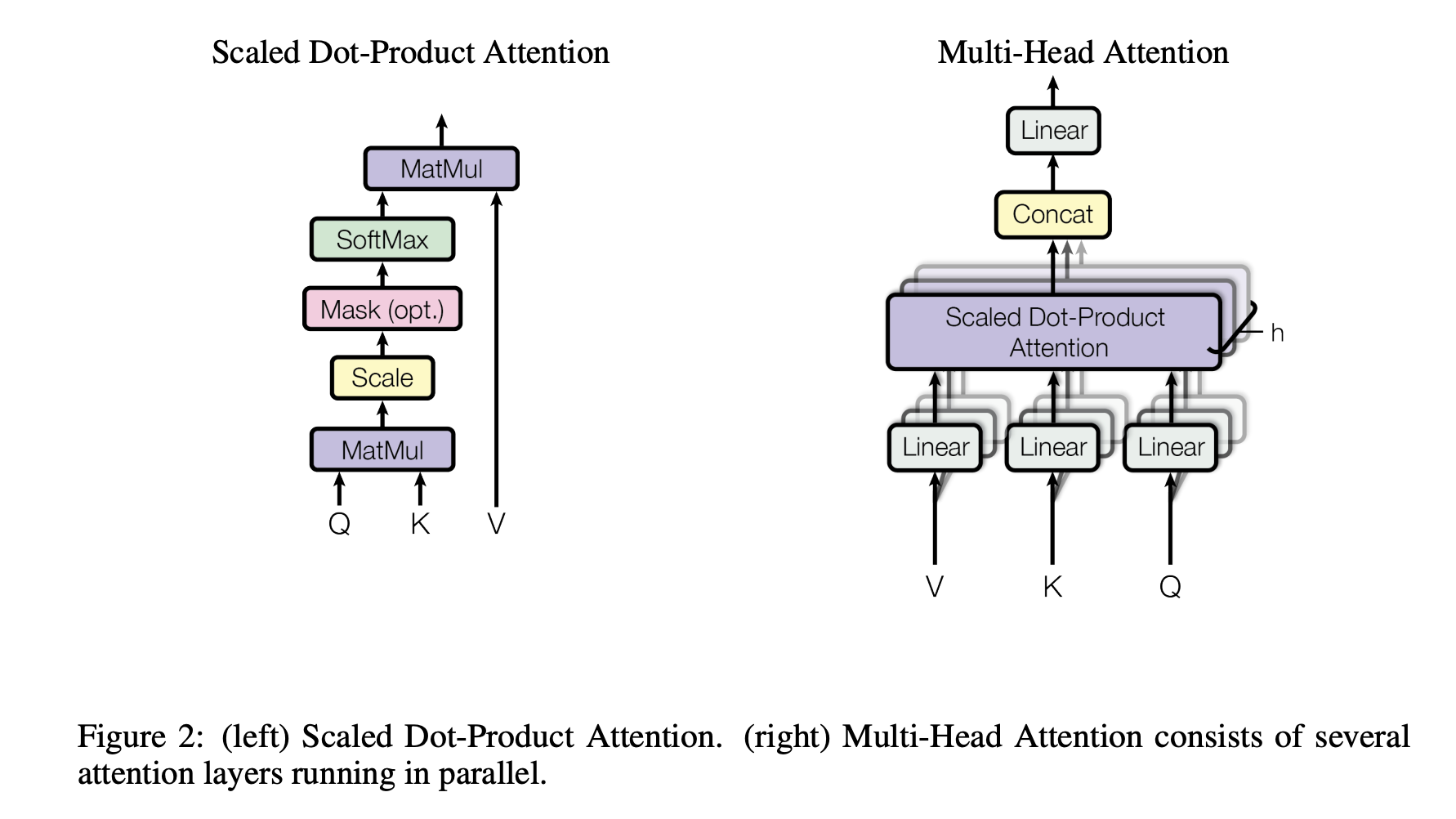
Scaled Dot-Product Attention

Scaled Dot-Product Attention에서 Attention 연산의 입력은 세 종류의 벡터(Q, K, V)로 구성됨. Query와 Key는 서로 내적을 해야 하므로 same dimension dₖ가짐. 하지만, Value는 weight sum의 대상이기 때문에 다른 dimension dᵥ를 가져도 됨. 결과적으로는 각 Query 벡터를 모든 Key 벡터와 내적해 유사도 점수를 계산하고, 그 점수들이 dimension이 커질수록 과도하게 커지는 것을 막기 위해 √dₖ로 나눈 다음, softmax를 적용하여 각 Value가 얼마나 중요한지를 나타내는 weight를 만듦.

 

In practice, we compute the attention function on a set of queries simultaneously, packed together into a matrix Q. The keys and values are also packed together into matrices K and V. → Query를 따로따로 계산하지 않고 하나의 행렬 Q로 묶어서 동시에 처리함. → Key와 Value도 마찬가지로 행렬로 묶어서 계산함. → Scaled Dot-Product Attention은 additive attention보다 더 빠르고 공간적으로 효율적임(space-efficient).

 

Dimension이 작을 때에는 additive attention과 scaled dot-product attention이 비슷함. → 다만, dimension이 커지면 additive attention이 scaling을 적용하지 않은 scaled dot-attention을 능가할 수는 있음. scaled dot-attention에서 dimension이 커지면 내적 값이 과도하게 커지고 혹은 과도하게 작아질 수 있음. 그렇게 되면 softmax의 gradient가 거의 0인 영역으로 진입함. 그래서 √dₖ로 scaling을 해주고 진행을 하는 것임.

 

그러면 왜 additive를 버리고 scaled-dot-attention을 택한거지?

기존의 dot-attention에 scale을 적용한 scaled-dot-attention이 additive attention과 성능이 거의 동일하면서도 훨씬 빠르고 병렬화에 최적화되어있어서 scaled-dot-attention을 적용함.

 

Multi-Head Attention

Instead of performing a single attention function with d_model-dimensional keys, values and queries, we found it beneficial to linearly project the queries, keys and values h times with different, learned linear projections to dk, dk and dv dimensions, respectively. → d_model인 상태로 512 dimension으로 attention을 한 번만 진행할 수도 있지만, Transformer에서는 Query, Key, Value 각각을 서로 다른 h개의 선형 변환(linear projection)으로 나눠서 변환하는 것이 더 좋다는 것을 발견함. 이때 각 projection은 학습되는 가중치를 가짐.

• 각 head마다
  • Query → dₖ 차원
  • Key → dₖ 차원
  • Value → dᵥ 차원
  • 하나의 큰 벡터를 여러 개의 head로 나눠 보는 구조임.

On each of these projected versions of queries, keys and values we then perform the attention function in parallel, yielding dv-dimensional output values. → 위에서 서로 다른 h개의 linear projection으로 분리한다고 하였으니까, 분리된 각 head마다 Scaled Dot-Product Attention을 independent하고 parallel하게 수행. → head 하나당 출력은 dᵥ 차원의 벡터, 총 h개의 출력이 동시에 만들어짐. 어쨌든, Attention의 weighted sum은 Value의 공간에 있으므로, 출력 차원은 dᵥ가 되는 게 맞음. → 즉, attention을 하나로 크게 하는 게 아니라 작은 attention(head, linear projection)을 여러 개 병렬로 수행한다고 보면 됨.

 

These are concatenated and once again projected, resulting in the final values, as depicted in Figure 2. → concat해서 다시 한 번 linear projection을 진행함(512 dimension).

 

Multi-head attention allows the model to jointly attend to information from different representation subspaces at different positions. With a single attention head, averaging inhibits this. → Multi-head의 장점에 대해서 조금 설명을 하고 있는데, 어떤 head는 문법적 관계에, 어떤 head는 의미적 유사성에, 어떤 head는 멀리 떨어진 토큰에 attention을 할 수 있음. 즉, 모델이 서로 다른 표현 공간(representation subspace)과 서로 다른 위치(position)를 동시에 바라볼 수 있게 됨. → uni-attention으로 하면 모든 관계를 하나의 weighted sum으로 처리하기 떄문에 다양한 관계 정보가 뭉개질 수 있음(resolution 저하.).

Multi-Head Attention

MultiHead(Q, K, V) = Concat(head₁, …, headₕ)Wᴼ → head₁부터 headₕ까지 h개의 attention 결과를 만들고 그 결과들을 옆으로 이어붙인 다음(concat) 마지막으로 선형 변환 Wᴼ을 한 번 더 해서 최종 출력으로 만듦.

headᵢ = Attention(QWᵢ^Q, KWᵢ^K, VWᵢ^V) → i번째 head에서는 Q를 Wᵢ^Q로 선형 변환, K를 Wᵢ^K로 선형 변환, V를 Wᵢ^V로 선형 변환. 그렇게 변형된 Q,K,V로 attention을 하나 수행. 각 head마다 Wᵢ^Q, Wᵢ^K, Wᵢ^V가 전부 다름.

투영 차원

• Wᵢ^Q ∈ ℝ^{d_model × d_k}
• Wᵢ^K ∈ ℝ^{d_model × d_k}
• Wᵢ^V ∈ ℝ^{d_model × d_v}
• 원래 Q, K, V는 전부 d_model 차원, 각 head에서는 이걸: Q, K → d_k 차원, V → d_v 차원으로 줄여서 봄.
• Q (512) → Wᵢ^Q → Qᵢ (64)
  K (512) → Wᵢ^K → Kᵢ (64)
  V (512) → Wᵢ^V → Vᵢ (64)
• Attention의 output은 V의 weighted sum이기 때문에 output dimension = value dimension = d_v

multi-head attention flow

입력 Q,K,V (512차원)
   ↓
8개의 서로 다른 선형 변환
   ↓
8개의 attention (64차원씩), 8 heads
   ↓
concat → 512차원
   ↓
선형 변환 Wᴼ
   ↓
최종 출력 (512차원)

 

결과적으로는 표현력은 여러 head 덕분에 커지고계산량은 single-head(512차원)와 거의 동일함.

 

Applications of Attention in our Model

Transformer는,

(1) Decoder가 Encoder 출력을 참고하는 encoder–decoder attention,

(2) Encoder 내부에서 모든 위치가 서로를 보는 self-attention,

(3) Decoder 내부에서 과거만 보도록 제한된 masked self-attention

이렇게 세 가지 방식으로 multi-head attention을 사용함.

 

Position-wise Feed-Forward Networks

In addition to attention sub-layers, each of the layers in our encoder and decoder contains a fully connected feed-forward network, which is applied to each position separately and identically. → attention 말고도 FFN이 들어가 있는데, 각 토큰 위치(position)에 대해서 서로 독립적으로(separately) 적용되고 모든 위치에서 같은 함수(identically)를 사용함. 같은 위치에서는 같은 parameter가 공유되지만 layer 사이에는 다른 parameter가 공유됨.

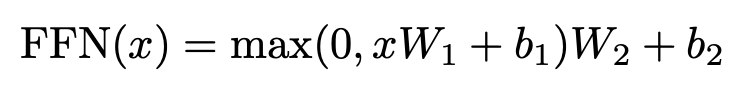
두 번의 linear transformation이 들어감 + ReLU.

 

Positional Encoding

Since our model contains no recurrence and no convolution, in order for the model to make use of the order of the sequence, we must inject some information about the relative or absolute position of the tokens in the sequence. → RNN, CNN과는 다르게 Transformer에서 self-attention은 순서를 전혀 모름. 그렇기 때문에, 이 단어가 앞에 있는지, 뒤에 있는지, 혹은 몇 번째 위치에 있는지 모름. 그렇기에 위치(position)에 대한 정보를 외부에서 injection을 해주어야 함.

To this end, we add "positional encodings" to the input embeddings at the bottoms of the encoder and decoder stacks.

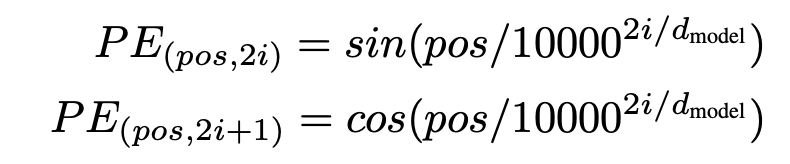
We chose this function because we hypothesized it would allow the model to easily learn to attend by relative positions. → 위치가 pos에서 pos+k로 이동하면 새로운 positional encoding은 기존 positional encoding의 선형 결합(linear function)으로 표현 가능함.

 

4. Why Self-Attention

1. 층 layer 당 계산 복잡도가 유리함.

• Self-attention은 한 층에서 모든 위치를 한 번에 연결함.
• RNN은 시퀀스 길이 n만큼 순차적으로 계산(O(n))해야 함.
• 문장 처리에서는 보통
  • 시퀀스 길이 n < 표현 차원 d (ex. n=50, d=512)
• 이 조건에서는 self-attention이 RNN보다 계산적으로 더 빠름.

2. 병렬화에서 성능이 뛰어남.

• Self-attention:
  • 모든 토큰 간 연산을 동시에 병렬 처리 가능.
  • 순차 연산 단계 수 = 상수(constant)
• RNN:
  • 이전 토큰 결과 없이는 다음 토큰 계산 불가.
  • 순차 연산 단계 수 = O(n)

3. Long range dependency에 대한 학습 성능이 뛰어남.

• Self-attention:
  • 어떤 두 위치든 한 번에 직접 연결
  • 최대 경로 길이 = O(1)
• RNN:
  • 앞에서 뒤까지 순차 이동
  • 최대 경로 길이 = O(n)
• CNN:
  • 커널 크기에 따라 여러 층 필요
  • 최대 경로 길이 = O(n/k) 또는 O(log n)
• Long range dependency 학습에서는 self-attention이 가장 유리함.

4. CNN과 비교했을 때 계산 효율이 Not Bad.

• 일반 convolution은:
  • 커널 폭 k만큼 연산 비용 증가.
  • RNN보다도 비쌀 수 있음.
• Separable convolution을 써도:
  • 복잡도는 여전히 큼.
• 심지어 k = n(전체 문장)인 경우:
  • self-attention + FFN 조합과 계산 복잡도가 동일.

5. Training

Optimizer를 다음과 같이 적용함. Adam 옵티마이저 사용. → 학습률은 고정은 아니지만, step에 따라 변함. → 초반 4000 step은 선형 증가(warmup). → 이후에는 1/√step로 감소. → 모델 차원(d_model)이 클수록 학습률은 작게 조정.

•  

•