[Paper Review] CVPR 2016, Learning Deep Features for Discriminative Localization 논문리뷰

Learning Deep Features for Discriminative Localization

CVPR 2016

• 논문 링크: https://arxiv.org/abs/1512.04150

0. Abstract

Shed light on how it explicitly enables the convolutional neural network to have remarkable localization ability despite being trained on image-level labels. → Global average pooling(GAP)의 구조적인 의미를 재발견하는 걸로 이해하면 됨. 논문에서도 remarkable localization이라고 해놨으니까 뭔가 이미지 내에서 위치를 알려주는 걸로 이해하면 됨.

 

While this technique was previously proposed as a means for regularizing training, we find that it actually builds a generic localizable deep representation that can be applied to a variety of tasks. → 원래 Global average pooling이 fully connected layer의 단점을 보완하고자 나온 건데(regularization을 통한 복잡도 줄이기), 다양한 task에 적용이 가능한 localization representation을 찾았다는 말임.

 

We demonstrate that our network is able to localize the discriminative image regions on a variety of tasks despite not being trained for them. → localization task를 학습시키지 않음에도 불구하고 localization이 가능하다는 뜻임. 그니까 모델은 classification만 학습을 함(localization task로 학습되지 않음.). 그럼에도 discriminative한 region을 찾음.

 

1. Introduction

Despite having this remarkable ability to localize objects in the convolutional layers, this ability is lost when fully-connected layers are used for classification. → CNN이  loacalization 능력이 있었지만, fully connected layer가 쓰임에 따라서 잊혀짐. Fully connected layer는 feature map을 flatten을 함에 따라서 공간 구조가 무너질 수 있음.

 

근데 요근래 neural network들(Network in Network(NIN) and GoogLeNet)은 fully connected layer를 피하려고 함. 왜 피하려고 하냐면 계산량의 문제 때문일 것 같은데 논문에서도 다음과 같이 설명함 'minimize the number of parameters while maintaining high performance.' → 이를 위해서 Global average pooling을 사용 which acts as a structural regularizer.

 

In our experiments, we found that the advantages of this global average pooling layer extend beyond simply acting as a regularizer - In fact, with a little tweaking, the network can retain its remarkable localization ability until the final layer.

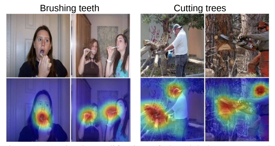
A CNN trained on object categorization is successfully able to localize the discriminative regions for action classification as the objects that the humans are interacting with rather than the humans themselves. → CNN을 object classification으로 학습을 진행, 그 모델을 action recognition에 적용, CAM으로 important region을 시각화를 했는데 tennis playing같은 행동에서 model은 사람이 아니라 tennis racket을 강조함. → 행동을 구분하는 데에 있어서 중요한 단서는 객체라고 할 수 있음.

 

Weakly-supervised object localization → 이해를 해보면, 가령 이미지는 dog인데 dog를 구별할 수 있는 discriminative한 bounding box는 어디있는지 모름. 즉 위치 정보는 주지 않고, class 정보만 준 상태라고 할 수 있음. 근데 이제 CAM에서는 이걸로 localization까지 하니까 Weakly-supervised object localization이라고 할 수 있음.

 

We use class activation map to refer to the weighted activation maps generated for each image, as described in Section 2.

 

We would like to emphasize that while global average pooling is not a novel technique that we propose here, the observation that it can be applied for accurate discriminative localization is, to the best of our knowledge, unique to our work. → GAP을 제안한 건 아니지만 GAP을 이용하여 뭔가 discriminative localization을 할 수 있다는 것으로 novelty를 찾음.

 

By removing the fully-connected layers and retaining most of the performance, we are able to understand our network from the beginning to the end → 아마 fully connected layer 대신에 GAP을 써서 사용할 것임.

 

Unlike [14] and [4], our approach can highlight exactly which regions of an image are important for discrimination.

 

2. Class Activation Mapping

 

In this section, we describe the procedure for generating class activation maps (CAM) using global average pooling (GAP) in CNNs. A class activation map for a particular category indicates the discriminative image regions used by the CNN to identify that category (e.g., Fig. 3).

 

We use a network architecture similar to Network in Network [13] and GoogLeNet [24] - the network largely consists of convolutional layers, and just before the final output layer (softmax in the case of categorization), we perform global average pooling on the convolutional feature maps and use those as features for a fully-connected layer that produces the desired output (categorical or otherwise). → Fully connected layer 자체를 없애겠다는 소리가 아니라 구조를 조금 변형해서 GAP을 사용하겠다는 의미임. 그러니까 Flatten + 대규모 FC 블록 ❌ / GAP + 작은 linear layer ⭕️ 이렇게 이해하면 될 듯함.

 

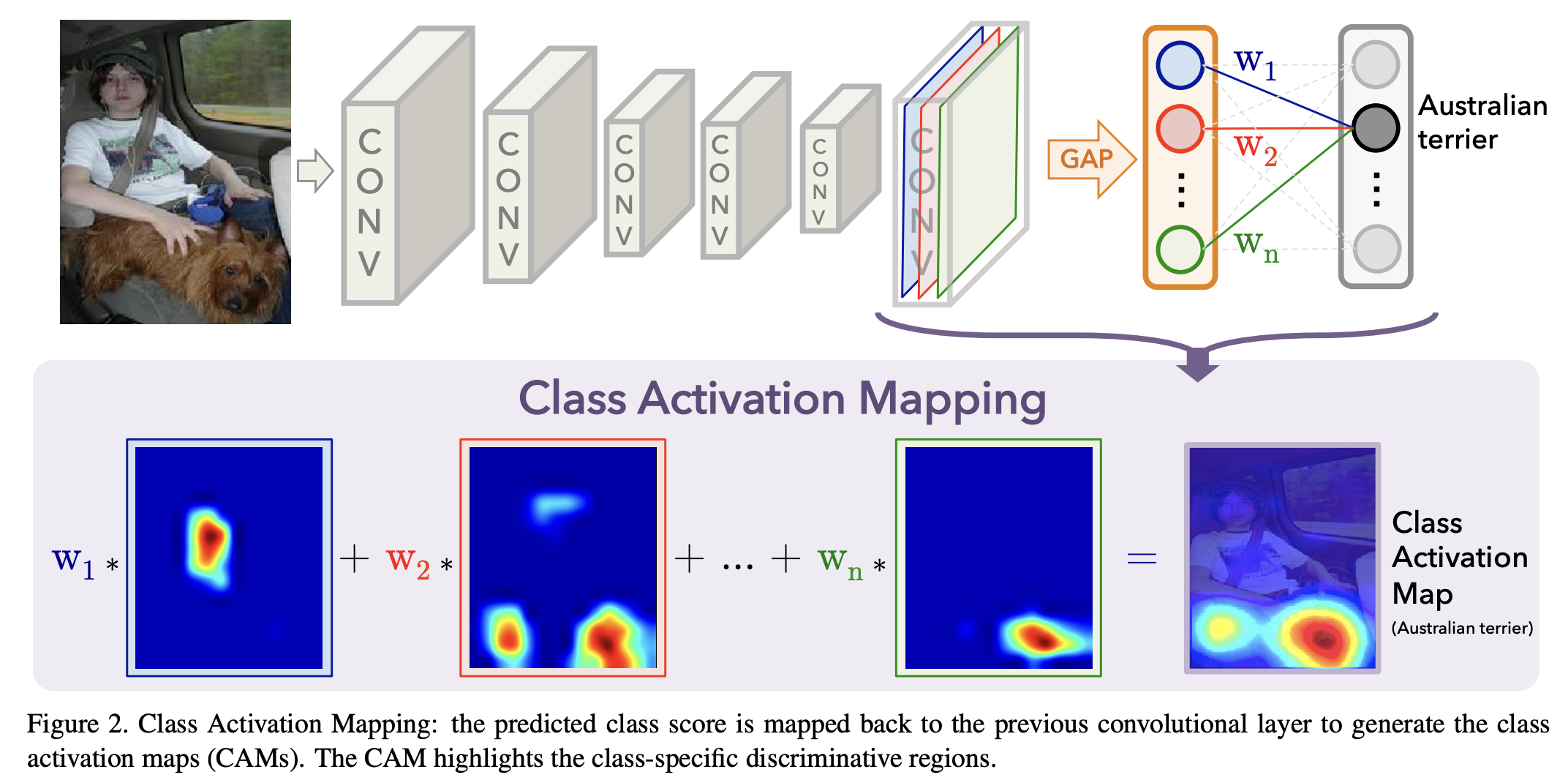
As illustrated in Fig. 2, global average pooling outputs the spatial average of the feature map of each unit at the last convolutional layer. A weighted sum of these values is used to generate the final output.

 

Class activation maps (CAM)의 수식 흐름을 보면 다음과 같음.

Input image에 대해 마지막 convolution layer의 출력을 다음과 같이 정의함.

각 채널 $k$의 공간 위치 $(x,y)$에서의 activation을 $f_k(x,y)$. 이는 마지막 convolution layer에서 feature map $k$가 위치 $(x,y)$에서 얼마나 활성화되었는지를 의미함.

 

여기서 채널 $k$에 대한 의미가 조금 와닿지가 않아서 채널 $k$에 대해서 조금 더 정리를 해보고 넘어가고자 함.

마지막 convolution layer의 output은 보통 $H \times W \times K$ 형태임. 여기서 $H, W$ → 공간 크기, $K$ → 채널 수 (feature map 개수), 여기서 $k$는 몇 번째 feature map인지를 나타내는 인덱스임. 즉, $k=1$ → 첫 번째 feature map, $k=2$ → 두 번째 feature map 으로 이해하면 될듯함. 그래서 정리해보면 $f_k(x,y)$는 $k$번째 feature map의 위치 $(x,y)$에서의 숫자 값임. 즉, 이 위치에서 특정한 패턴이 얼마나 강하게 반응했는가를 나타내는 값임.

 

다시, CAM으로 넘어와보면, 채널 $k$에 대해 global average pooling을 수행한 결과는 $F_k = \sum_{x,y} f_k(x,y)$임. 

 

즉, feature map $k$의 모든 공간 위치에서의 activation을 합산한 값임. $F_k$는 해당 패턴이 이미지 전체에서 얼마나 강하게 나타나는지를 나타냄.

 

한편, 클래스 $c$에 대한 softmax 입력값(=logit)은 $S_c = \sum_k w_k^c F_k$로 정의됨. 여기서 $w_k^c$는 클래스 $c$에 대해 유닛 $k$가 가지는 가중치이고, 이는 클래스 $c$를 예측할 때 feature $k$가 얼마나 중요한지를 나타냄.

 

즉, $w_k^c$는 $F_k$의 클래스 $c$에 대한 중요도를 의미함.

 

클래스 $c$의 최종 확률은 $P_c = \frac{\exp(S_c)}{\sum_c \exp(S_c)}$로 계산됨. 이는 각 클래스 점수 $S_c$를 확률로 변환한 값임.

 

계산 과정에서의 핵심은 다음과 같음. 분류 점수 $S_c$는 전역 평균된 feature $F_k$들의 가중합으로 표현됨. 이 선형 구조가 이후 $M_c(x,y) = \sum_k w_k^c f_k(x,y)$ 형태의 Class Activation Map으로 이어짐.

 

이어서, 앞에서 $F_k$는 $k$번째 feature map을 GAP로 요약한 값, $S_c$는 클래스 $c$의 점수(logit)의 내용을 정리했음.

 

여기서 $F_k = \sum_{x,y} f_k(x,y)$를 클래스 점수 식 $S_c = \sum_k w_k^c F_k$에 대입을 하게 되면,  $S_c = \sum_k w_k^c \sum_{x,y} f_k(x,y)$ 식을 도출할 수 있음.

 

다만, 여기서 순서를 바꿀 수 있는데 위 수식은 채널 $k$부터 돌면서, 그 안에서 공간 $(x,y)$를 다 더한다로 이해할 수 있는데 합 자체는 순서를 바꿀 수 있으므로, 순서를 바꿔서 다음과 같은 수식을 도출할 수 있음. $S_c = \sum_{x,y} \sum_k w_k^c f_k(x,y)$

 

즉, "채널 $k$부터 돌면서, 그 안에서 공간 $(x,y)$를 다 더함" → "먼저 위치 $(x,y)$를 하나 잡고 그 위치에서 모든 채널 $k$의 contribution를 합치고 그걸 모든 위치에 대해 더함." 이렇게 하면 CAM을 정의할 수 있음.

 

위 논문의 저자는 클래스 $c$에 대한 Class Activation Map을 다음과 같이 정의함. $M_c(x,y) = \sum_k w_k^c f_k(x,y)$

 

이걸 이해해보면 위치 $(x,y)$에서 feature map들의 activation $f_k(x,y)$를 클래스 $c$의 가중치 $w_k^c$로 가중합한 값이라고 이해할 수 있고, $M_c(x,y)$가 바로 heatmap의 픽셀 값(또는 격자 값)이 됨.

 

그래서 위에서 합 순서를 바꾼 식과 $M_c(x,y)$ 정의를 보면, $S_c = \sum_{x,y} M_c(x,y)$가 됨. 즉, CAM $M_c(x,y)$를 공간 전체에서 다 더하면 클래스 점수 $S_c$가 된다는 관계가 성립함.

 

CAM을 총정리해보면, $M_c(x,y)$ 값이 큰 위치는 “클래스 $c$ 점수를 올리는 데 크게 기여한 위치”임. 반대로 작거나 음수면 “클래스 $c$에 도움이 안 되거나 방해되는 위치”로 이해할 수 있음.

 

그래서 $M_c(x,y)$를 시각화하면 모델이 클래스 $c$를 판단할 때 무엇을 근거로 봤는지 명확하게 알 수 있음.

6. Conclusion

In this work we propose a general technique called Class Activation Mapping (CAM) for CNNs with global average pooling. This enables classification-trained CNNs to learn to perform object localization, without using any bounding box annotations.